This post is a summary of our latest paper [1] on improving an urban climate model to better predict building energy consumption depending on local weather conditions, the structure of buildings and human behaviours.
The paper is available online here. Get in contact if you would like a copy from me.
First, a little bit of background…
Weather changes energy use
We use more electricity and other forms of energy during very hot and cold weather. That’s because a lot of total energy is used to maintain comfortable temperatures inside buildings.
Below are scatter plots of the relationship between energy use in the state of Victoria and daily maximum air temperatures in Melbourne. When air temperatures drop, more gas is used for heating, and when air temperatures rise, more electricity is used for cooling.
Energy use (Victoria) and air temperature (Melbourne) for the period 2000-2009, with weekends removed. Energy use is scaled to Watts per square metre based on the population density of Preston. Click on legend to isolate data.
Energy use changes weather
Conversely, energy use changes the weather. That’s because nearly all energy used ends up as waste heat emitted into the atmosphere. Think of the heat coming off the back of your computer, but for every device, air conditioner, vehicle etc. Not only does this measurably increase air temperatures in cities, the injection of heat into the lower atmosphere causes convection, like a pot of water on a stove. That can change buoyancy driven atmospheric flows, affecting winds, precipitation and air quality (see previous post here).
So building energy consumption and urban climate are interlinked. Having a model which can represent their interactions improves our understanding of environmental processes and allows us to study local conditions and energy use under different scenarios.
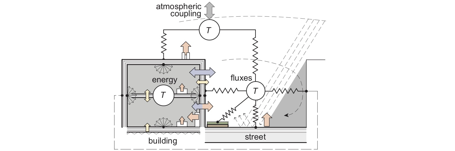
Although there are many neighbourhood to city-scale environmental models, only a small number can both dynamically predict energy consumption and are efficient enough to be used as a land surface in regional or global climate model simulations. And as far as I know, there aren’t any other models that have been designed specifically for Australian conditions. To help fill this gap we developed the Urban Climate and Energy Model (UCLEM).
What we did
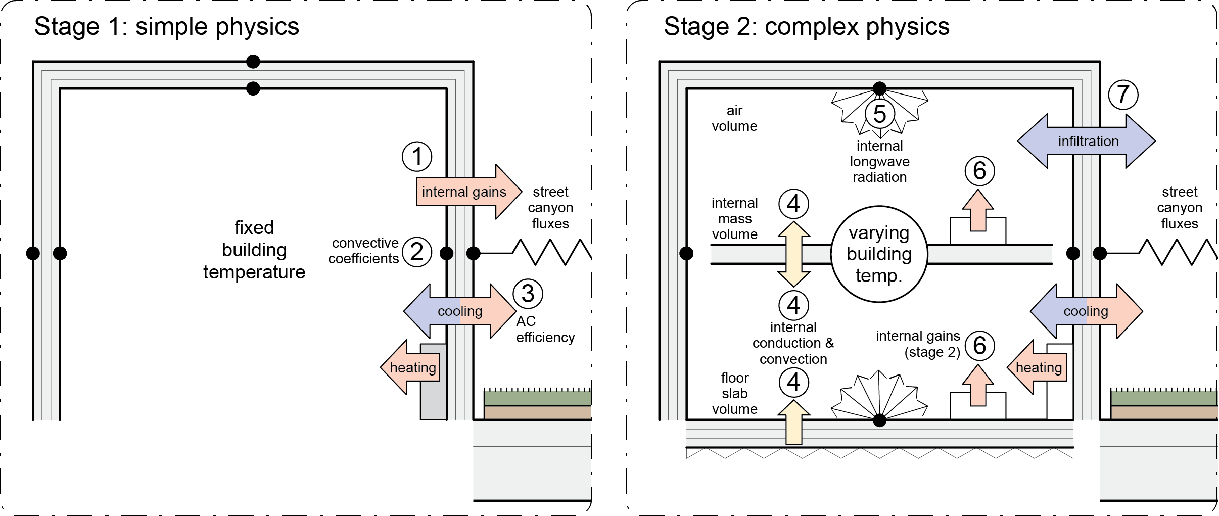
Starting with the Australian Town Energy Budget (aTEB) model [2], we added complexity in four stages to see what most improved energy demand predictions.
Stage 1 retained a very simple representation of buildings (just the outside envelope and a fixed internal air temperature) but a few processes were improved (e.g. air conditioning efficiency). This retained a fast and simple model, but is not very realistic.
Stage 2 introduced more internal/external heat transfer processes, including longwave radiation exchange, internal thermal inertia and exchange of air between inside and out (infiltration - very important for leaky Australian houses!).
Stage 3 introduced a representation of human behaviours by modulating energy use over the diurnal cycle based on electricity use data in Australia.
Stage 4 introduce more complex human behaviours, attempting to represent differences in tendencies to control temperature.
Each stage was evaluated on its ability to reproduce observed energy use (electricity and gas combined) every half hour for a 12-month period, with the model being subjected to near-surface meteorological observations.
To fairly compare each stage, we used an objective procedure to shuffle and find the optimal sets of values describing physical parameters (within a realistic range) which resulted in the lowest possible errors for each stage individually. I’ve described this procedure in a previous post here.
Results
The figure below shows the daily average energy use (solid lines) with the daily ranges (shading) in each Stages 1, 2 3 and 4, with the original model (Stage 0) in blue in the first panel. Each red line plots the best performing simulation at that stage.
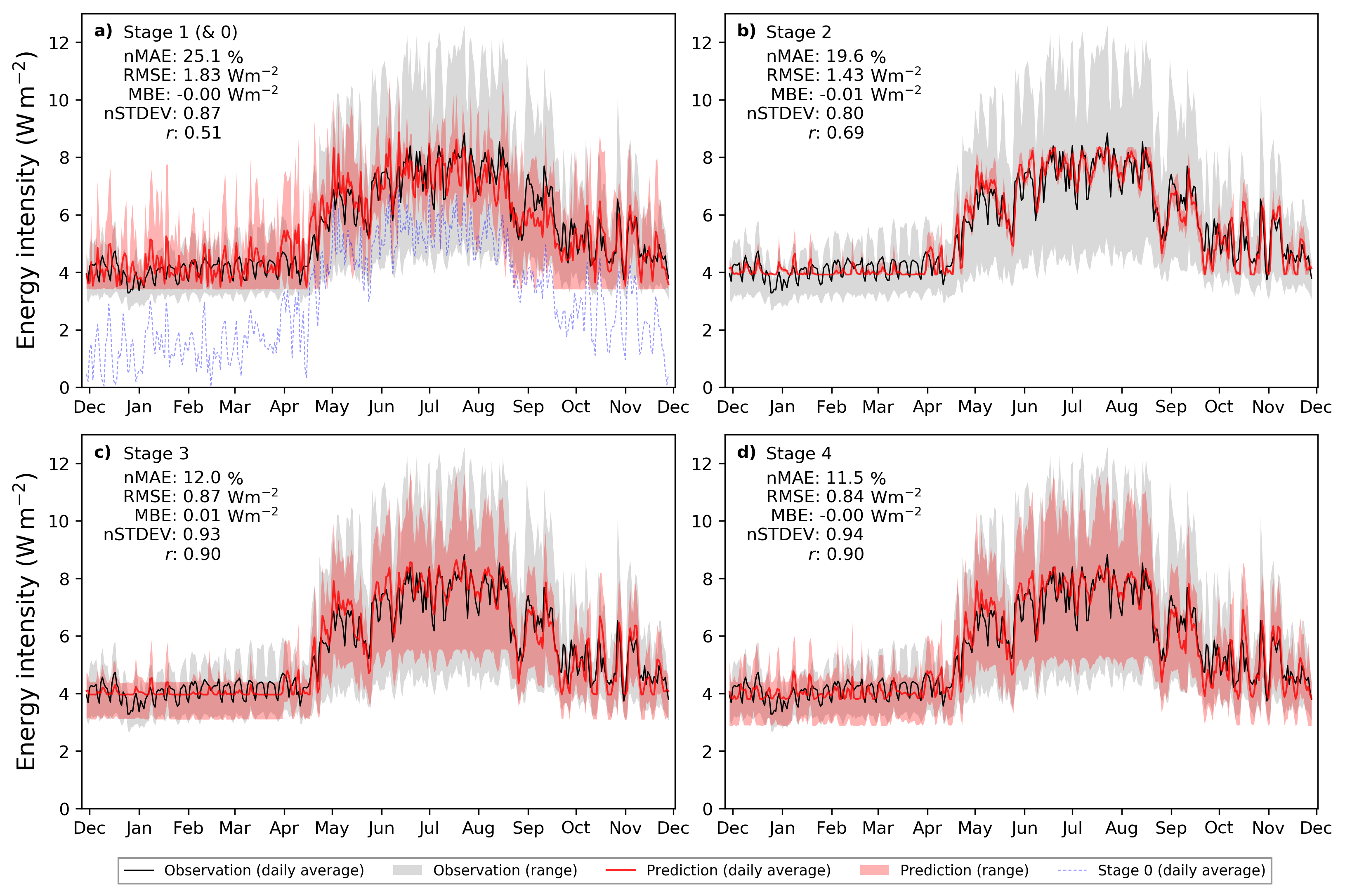
Initially, Stage 0 had a normalised mean absolute error of 56.5% (nMAE: the average prediction error far each half hour over 12 months as a proportion of the mean of all observed values). This large error was primarily because the original model was not designed as a building energy model, so it didn’t include energy used by non-heating/cooling electrical and gas appliances (like TVs, lights etc).
Stage 1 introduces an estimate of those other devices, along with some other minor changes, and model errors are halved to 25.1% (see figure panels).
Stage 2 with more complex internal physics reduces errors to 19.6%. It quite accurately predicts how average daily energy use differs between days and seasons, but fails to predict the observed daily range of energy use.
It is not until the introduction of human behaviours in Stage 3 that predicted daily ranges start to match observed ranges, and errors are reduced to 12.0%. These human behaviours are based on a statistical model derived from the national electricity networks[3]. This is described in more detail below.
Finally, a more complex representation of human behaviours in Stage 4 only slightly improves results over Stage 3, down to a 11.5% average error. The additional complexity probably doesn’t justify the small additional improvement over Stage 3.
Although there is now quite a good match there are still some problems, for example the mismatch during warmer months. We’ve continued development since publishing, for example by allowing for the observed drop in energy use on weekends, and improved results further since then.
Representing human behaviours
Compared with others, this model does do quite few things differently in representing the physical environment, but I think the most interesting feature is the novel way in which human behaviour is represented.
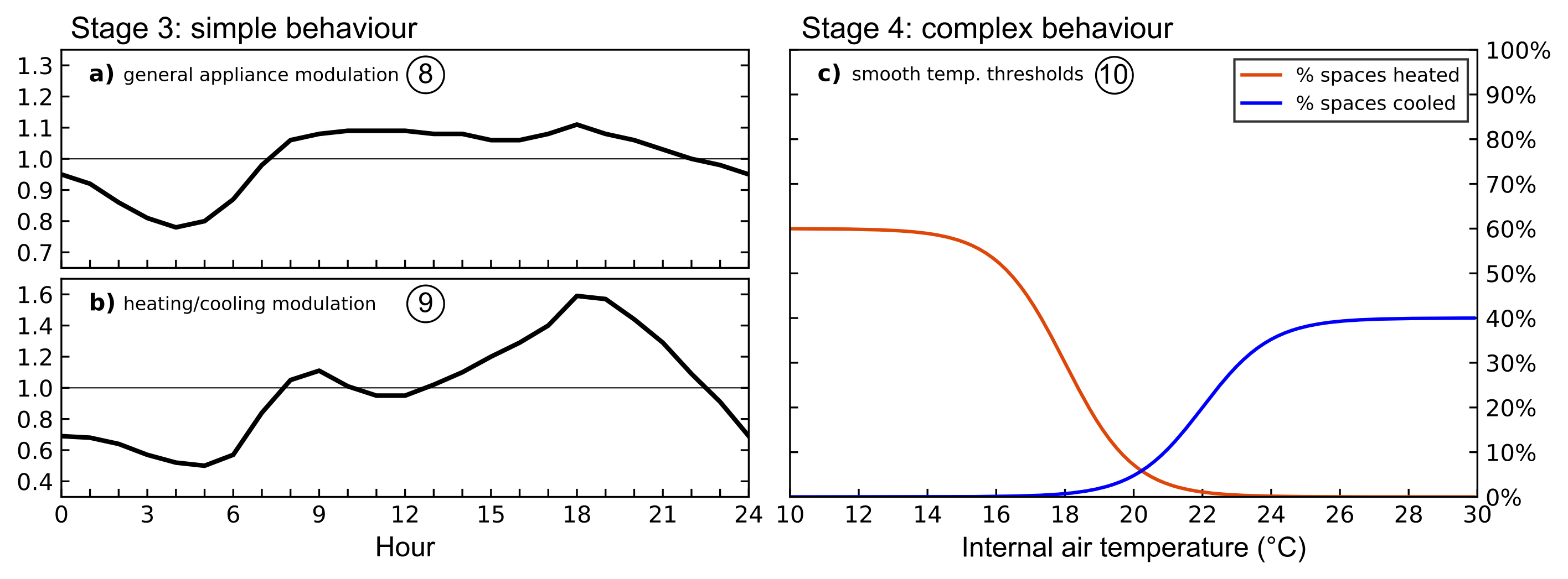
Stage 3 introduces a modulation of energy use over the diurnal cycle based on a previously developed statistical model[3], which helpfully separated the different way that temperature dependent devices (heaters and air-conditioners) and all other energy devices (TVs, computers, lights etc.) were being used. The modulation of energy use over a diurnal cycle are representative of an average of all behaviours within the spatial area of energy use data - in this case the State of Victoria.
This kind of aggregated behavioural information is useful in a model like UCLEM which is intended not to represent a single building or single occupant’s behaviour, but the average of many buildings together. This represents a simple way to capture average human behaviour, and is more objective and straightforward than the common method of creating a series of timing schedules which represent behaviours (e.g. a time at which an air-conditioner gets turned on).
I will write an additional post to describe the statistical model in more detail at a later date.
So what?
So the model is able to recreate the energy used in Melbourne back in 2004. So what? Unlike a purely statistical model this model includes a description of the physical nature of the city - building heights, street widths, trees, wall, roof and floor materials, surface albedo etc etc. This means that we can undertake experiments to examine how energy use or urban climate will change if we make interventions into the built environment - or if interventions are forced upon it.
So, with this model you could ask things like:
- how would urban climate and energy use change in a higher density city?
- How much can green space reduce urban heat in different regional climates and in different weather events?
- how will electricity use change under IPCC global warming scenarios?
- how much do air-conditioners blowing heat into streets actually raise urban air temperatures?
- will painting all roofs white reduce urban air temperatures, or will that reduce convection and air flow and make things even more uncomfortable?
Because the tool is fast, flexible and can form a component of a regional or global climate model, the research opportunities are very broad.