Our new paper brings together 20 urban flux tower sites from around the world into a harmonised, gap filled, quality controlled collection. The collection is openly available. Read more by clicking here.
There are thousands of flux towers in natural areas, and much of the data they have collected are openly avalable through programs such as FLUXNET and OzFLUX. But as far as we are aware, only a single urban site had previously been included in these open collections.
Flux tower observations are critical for understanding how land and atmosphere interact, and help to evaluate the processes we represent in weather and climate models.
Establishing and maintaining long-term flux sites in cities is challenging because of the complex terrain (which requires higher and more expensive towers), difficulty in gaining approval and extremely limited long-term funding opportunities for urban sites. So we worked with 25 observational co-authors to establish, for the first time, an open urban-focussed collection. This is a big deal for the urban climate research community, both for understanding fundamental interactions, and for helping develop better models of these interactions.
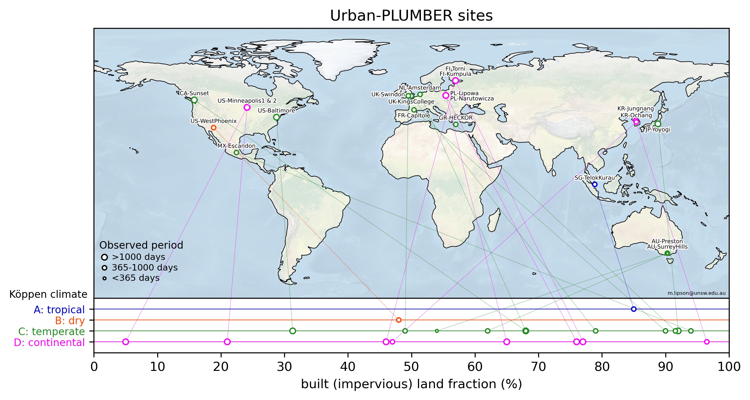
The 20 sites are diverse in urban characteristics and regional climate. Cities include Toulouse, Tokyo, Seoul, Mexico City, Amsterdam, Lodz, Baltimore, Minneapolis, Pheonix, Melbourne, Vancouver, Helisinki, Heraklion, Singapore, Swindon and London. However, large gaps remain (e.g. in Africa and South America). We need to work harder to fund long-term observations in fast growing and understudied urban regions with huge environmental challenges.
 |
 |
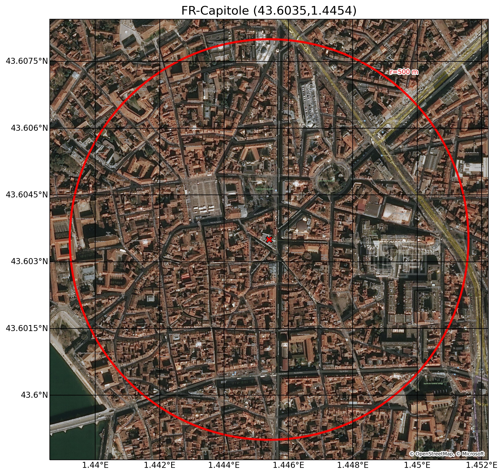
Each of the 20 sites have their own webpage with site characteristics, site images and plots, for example the FR-Capitole site in Toulouse, France, above. We collected these data to evaluate urban climate models in the Urban-PLUMBER model evaluation project, now underway.
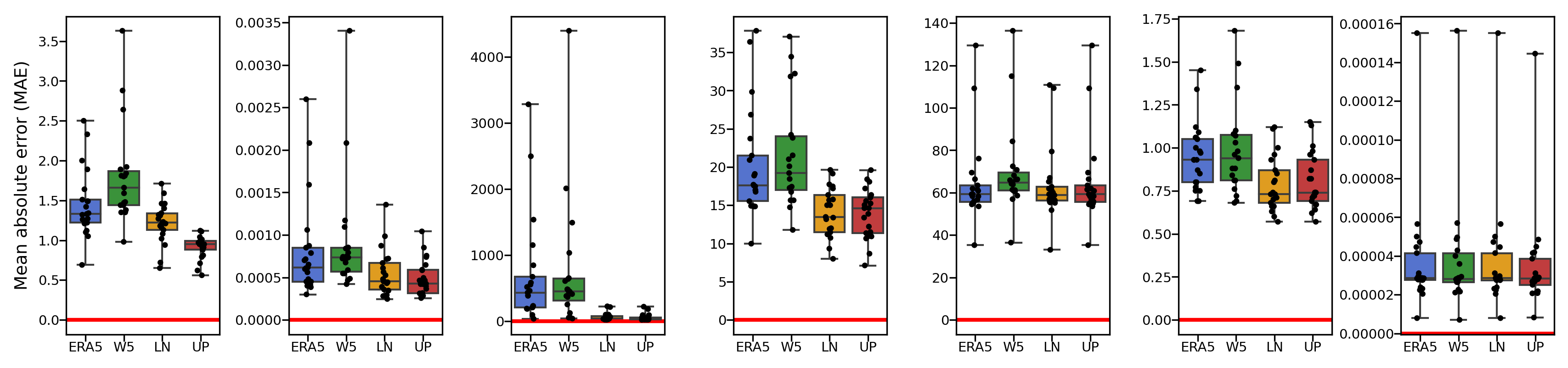
While the observations can have missing data (from equipment failure or quality control procedures), we need to fill gaps if using these data to drive land surface models. We used bias corrected ERA5 data, which is a “reanalysis” product available globally and at hourly timesteps. But as the underlying models in ERA5 don’t have any representation of urban areas, and the grid resolution is coarse compared with the flux tower footprint, we applied bias correction to help the ERA5 data better match conditions of the site. This bias correction method is novel, and had lower errors than other previously used methods.
This same method of bias-corrected ERA5 data allows us to include a 10-year “spin-up” period of locally appropriate synthetic data so that land surface models can equilibriate with local climate conditions.
The collection includes site characteristics data such as land cover fractions (buildings, roads, trees, grass etc.), building height and morphology, aerodynamic roughness estimates, population density and satellite imagery. The site data is included as csv and in netcdf files, so can be used to configure models. It’s also available from the project website: https://urban-plumber.github.io/sites
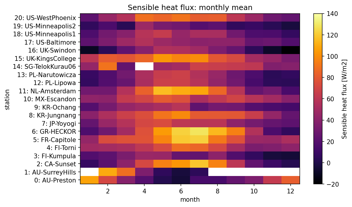
The 10-year spinup and gap filled forcing observation are available in text and netcdf formats. Also included is an “obs only” collection: a smaller subset of data useful for analysing observations. Data meet quality control, but are not gap filled, and are available in a single netcdf file allowing easy import and analysis. For example, the code below loads and plots the following plot.
import xarray as xr
import matplotlib.pyplot as plt

# open local standard time dataset and get monthly mean of sensible heat flux for each site
ds = xr.open_dataset('UP_all_clean_observations_localstandardtime_v1.nc')
grp = ds['Qh'].groupby('time.month').mean()

# plot mean value for each month and each station
fig,ax = plt.subplots(figsize=(8,5))
grp.plot(ax=ax,cmap='inferno', vmin=-20,vmax=140, cbar_kwargs={'label': 'Sensible heat flux [W/m2]'})
ax.set_title(f'Sensible heat flux: monthly mean')
ax.set_yticks(range(0,21))
ax.set_yticklabels([ds.station.station_ids[i] for i in range(0,21)])
fig.savefig('Qh_monthlymean.png', bbox_inches='tight', dpi=150)
Check out the paper here: Harmonized gap-filled datasets from 20 urban flux tower sites