This post describes how our interface conduction scheme is formulated and computed, and finishes with Fortran code which solves various approximations of the heat equation.

The heat equation

Conduction through a material is described by the heat equation, a combination of Fourier’s law and the conservation of energy. In one dimension they are:

$$ q = -\lambda \frac{\partial T}{\partial x},$$

$$ \rho c \frac{\partial T}{\partial t} = \frac{\partial q} {\partial x},$$

where $ q $ is local heat flux density , $ \lambda $ thermal conductivity, $ T $ is temperature, $ \rho c $ is volumetric heat capacity, in $ t $ time and $ x $ space dimensions.

In simple situations exact solutions can be found through analytic means. In more complex or real world situations where material and boundary conditions vary non-uniformly, then other methods are required.

Finite difference methods

Solutions to partial differential equations can be approximated with finite-difference methods, where a continuous function is discretised into approximate derivatives and solved numerically, for example:

$$ \frac{\partial T}{\partial t} \approx \frac{T^{t+\Delta t} - T^{t}}{\Delta t} .$$

Finite difference approximations include explicit (or forward time, centred space), implicit (backward time, centred space) and semi-implicit (Crank-Nicholson) methods.

• For explicit methods, the change to a system at the next timestep is based on the current state of the system. In other words, the change in a single variable can be calculated in a single equation, as relevant information is known explicitly and projected forwards. Explicit methods are easiest to implement and are computationally efficient, but can be unstable when projections too far overshoot the exact result.

• Implicit methods consider how a system will change over the timestep in question, so equations for each element in the system must be solved simultaneously. Implicit methods are harder to implement and compute, but they are always stable, allowing arbitrarily long timesteps.

• Semi-implicit schemes mix explicit and implicit methods, improving accuracy but are harder again to implement and compute, and can still be unstable depending on the degree of explicitness.

As our model is used for climate projects over long time periods, large timesteps are desirable to improve efficiency, hence we approximate the heat equation using fully implicit methods.

General implicit form

If we are to represent the heat equations in discrete form, we need to approximate conductivity and heat capacity into effective values between nodes. We can define effective parameters in various ways (two are described here), but the general form of the discretised equations remain the same. For the implicit form, we want the temperature gradient between nodes at the next timestep ($m+1$), so Fourier’s law becomes:

$$ q_{k \rightarrow} = \tilde{\kappa}_{k \rightarrow} \left( T_{k}^{m+1}-T_{k+1}^{m+1} \right),$$

where $ q_{k \rightarrow} $ is heat flux, and $\tilde{\kappa}_{k \rightarrow}$ effective conductance between node $ k $ and $k+1.$ Likewise, the conservation law becomes:

$$ \frac{\tilde {C}_k}{\Delta t} \left( T^{m+1}_k - T^m_k \right) = \left( q_{(k-1) \rightarrow} - q_{k \rightarrow} \right), $$

where $\tilde{C}_{k} $ is effective capacitance. Combining these equations, we have a discretised heat equation in general implicit form:

$$ \frac{\tilde {C}_k}{\Delta t} \left( T^{m+1}_k - T^m_k \right) = \tilde {\kappa}_{(k-1) \rightarrow } \left( T^{m+1}_{k-1} -T^{m+1}_k \right) - \tilde {\kappa}_{k \rightarrow} \left( T^{m+1}_k -T^{m+1}_{k+1} \right) . $$

Solving the implicit form

By collecting terms of the general implicit equation, we can describe the system as:

$$ a_k \left[ T_{k-1}^{m+1} \right] + b_k \left[ T_{k }^{m+1} \right] + c_k \left[ T_{k+1}^{m+1} \right] = d_k $$

where $d$ represents all remaining terms including the current temperature at node $k$. The system of equations can be represented in a matrix:

$$ \begin{bmatrix} b_1 & c_1 & \cdot & \cdot & \cdot & \cdot \\\ a_2 & b_2 & c_2 & \cdot & \cdot & \cdot \\\ \cdot & a_3 & b_3 & c_3 & \cdot & \cdot \\\ \cdot & \cdot & \ddots & \ddots & \ddots & \cdot \\\ \cdot & \cdot & \cdot & a_{n-1} & b_{n-1} & c_{n-1} \\\ \cdot & \cdot & \cdot & \cdot & a_n & b_n \end{bmatrix} \begin{bmatrix} T_1^{m+1} \\
T_2^{m+1} \\
T_3^{m+1} \\
\vdots \\
T_{n-1}^{m+1} \\
T_n^{m+1} \\
\end{bmatrix}=\begin{bmatrix} d_1 \\
d_2 \\
d_3 \\
\vdots \\
d_{n-1} \\
d_n \\
\end{bmatrix}. $$

A tridiagonal matrix of this type can be solved using Thomas algorithm, an efficient method of Gaussian elimination.

The Thomas Algorithm

A tridiagonal matrix over $n$ nodes is solved in the following steps. First, the forward elimination phase:

do, for k = 2nd step until n: $$ \begin{align} m &= \frac{a_k}{b_{k-1}} \\
b_k &= b_k - mc_{k-1} \\
d_k &= d_k - md_{k-1} \end{align} $$ end do

Then, the first step of the backward substitution phase: $$ T_{n}^{m+1} = \frac{d_n}{b_n} ,$$ afterwhich:

do, for k = n-1 down to 1: $$ T_k^{m+1} = \frac{d_k-c_kT_{k+1}}{b_k}. $$ end do

The $T^{m+1}$ vector now describes updated temperatures at each node.

Coefficients of the tridiagonal matrix

Consider a composite material of $n$ layers, each with different depths ($d$), conductivities ($\lambda$) and heat capacities ($c$). The boundary conditions are controlled by external and internal temperatures ($T_{ext}, T_{int}$), and surface thermal resistances ($R_{ext}, R_{int}$). The coefficients of the tridiagonal matrix will change depending on how the material is sliced into nodes, and how we represent effective conductance and capacitance. Here we consider three methods.

The standard half-layer scheme is described by a system of equations from $1$ to $n$:

$$ \begin{align}
a_1 &= n/a \\
a_{2..n} &= - \left[ \frac{1}{2} \left( \frac{d_{{k-1}}}{ \lambda_{{k-1}}} + \frac{d_{k}}{ \lambda_{k}} \right) \right]^{-1} \\
\\
b_1 &= \left[ R_{ext} + \frac{1}{2} \left(\frac{d_{1}}{ \lambda_{1}} \right) \right]^{-1} + \left[ \frac{1}{2} \left( \frac{d_{1}}{ \lambda_{1}} + \frac{d_{2}}{ \lambda_{2}} \right) \right]^{-1} + \frac{c_1 d_1}{\Delta t} \\
b_{2..n-1} &= \left[ \frac{1}{2} \left( \frac{d_{{k-1}}}{ \lambda_{{k-1}}} + \frac{d_{k}}{ \lambda_{k}} \right) \right]^{-1} + \left[ \frac{1}{2} \left( \frac{d_{k}}{ \lambda_{k}} + \frac{d_{k+1}}{ \lambda_{k+1}} \right) \right]^{-1} + \frac{c_k d_k}{\Delta t} \\
b_n &= \left[ \frac{1}{2} \left( \frac{d_{n-1}}{ \lambda_{n-1}} + \frac{d_{n}}{ \lambda_{n}} \right) \right]^{-1} + \left[ \frac{1}{2} \left( \frac{d_{n}}{ \lambda_{n}} \right) + R_{int} \right]^{-1} + \frac{c_n d_n}{\Delta t} \\
\\
c_{1..n-1} &= - \left[ \frac{1}{2} \left( \frac{d_{{k}}}{ \lambda_{k}} + \frac{d_{k+1}}{ \lambda_{k+1}} \right) \right]^{-1} \\
c_n &= n/a \\
\\
d_1 &= \frac{T_1^m c_1 d_1}{\Delta t} + \frac{T_{ext}}{ R_{ext} + \frac{1}{2} \left( \frac{d_{1}}{ \lambda_{1}} \right)} \\
d_{2..n-1} &= \frac{T_k^m c_k d_k }{\Delta t} \\
d_n &= \frac{T_n^m c_n d_n}{\Delta t} + \frac{T_{int}}{ \frac{1}{2} \left( \frac{d_{n}}{ \lambda_{n}} \right) + R_{int}} \\
\end{align} $$

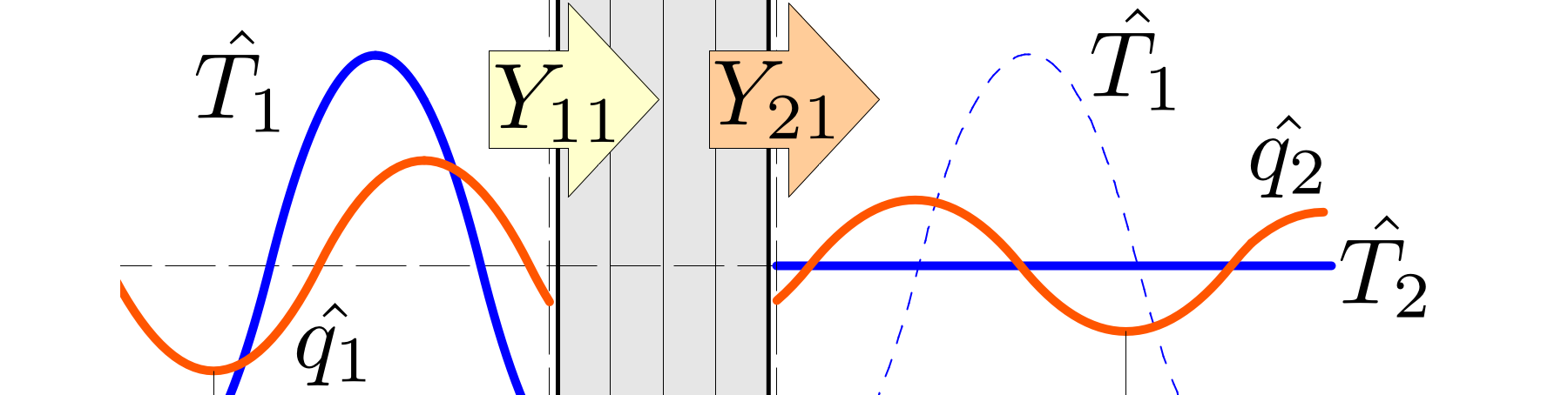
The interface scheme has an additional node, so is described by a system of $n+1$ equations. Here we shift the node indexes to extend from $0$ to $n$:

$$ \begin{align}
a_0 &= n/a \\
a_{1..n} &= - \frac{\lambda_{k}}{d_{k}} \\
\\
b_0 &= \frac{1}{R_{ext}} + \frac{\lambda_1}{d_1} + \frac{\tfrac{1}{2} \left( c_{1} d_{1} \right)}{\Delta t} \\
b_{1..n-1} &= \frac{\lambda_{k}}{d_{k}} + \frac{\lambda_{k+1}}{d_{k+1}} + \frac{\tfrac{1}{2} \left( c_{k} d_{k} + c_{k+1} d_{k+1} \right)}{\Delta t} \\
b_{n} &= \frac{\lambda_n}{d_n} + \frac{1}{R_{int}} + \frac{\tfrac{1}{2} \left( c_{n} d_{n} \right)}{\Delta t} \\
\\
c_{0..n-1} &= - \frac{\lambda_{k+1}}{d_{k+1}} \\
c_{n} &= n/a \\
\\
d_0 &= \frac{\tfrac{1}{2} \left( c_1 d_1 \right) T_1^m }{\Delta t} + \frac{T_{ext}}{ R_{ext}} \\
d_{1..n-1} &= \frac{\tfrac{1}{2} \left( c_{k} d_{k} + c_{k+1} d_{k+1} \right) T_k^m }{\Delta t} \\
d_{n} &= \frac{\tfrac{1}{2} \left( c_n d_n \right) T_n^m }{\Delta t} + \frac{T_{int}}{ R_{int}} \\
\end{align} $$

By inputing the coefficents from either scheme within the Thomas algorithm, an estimate of the temperature of each node at the next timestep can be calculated.

Modified half-layer scheme

A slight modification of the standard half-layer system is possible where an additional node is placed at the external skin of the system, allowing the temperature to be estimated there. If the additional node has zero heat capacity, then it is a purely diagnostic variable and does not affect other node temperatures or heat storage flux for the system as a whole.

Having an additional node at the surface of the system is useful as the skin temperature is needed to calculate the exchange of energy between the material and the external environment. In addition, the modification means both the interface and modified half-layer schemes have the same number of nodes ($n+1$), simplifying array allocation and matrix manipulation in code which includes both schemes.

The modified half-layer scheme is described by a system of $n+1$ equations, so again we shift the node indexes to extend from $0$ to $n$:

$$ \begin{align}
a_0 &= n/a \\
a_{1} &= - \left[ \frac{1}{2} \left( \frac{d_{{1}}}{ \lambda_{{1}}} \right) \right]^{-1} \\
a_{2..n} &= - \left[ \frac{1}{2} \left( \frac{d_{{k-1}}}{ \lambda_{{k-1}}} + \frac{d_{k}}{ \lambda_{k}} \right) \right]^{-1} \\
\\
b_0 &= \frac{1}{R_{ext}} + \left[ \frac{1}{2} \left( \frac{d_{1}}{ \lambda_{1}} \right) \right]^{-1} \\
b_1 &= \left[ \frac{1}{2} \left(\frac{d_{1}}{ \lambda_{1}} \right) \right]^{-1} + \left[ \frac{1}{2} \left( \frac{d_{1}}{ \lambda_{1}} + \frac{d_{2}}{ \lambda_{2}} \right) \right]^{-1} + \frac{c_1 d_1}{\Delta t} \\
b_{2..n-1} &= \left[ \frac{1}{2} \left( \frac{d_{{k-1}}}{ \lambda_{{k-1}}} + \frac{d_{k}}{ \lambda_{k}} \right) \right]^{-1} + \left[ \frac{1}{2} \left( \frac{d_{k}}{ \lambda_{k}} + \frac{d_{k+1}}{ \lambda_{k+1}} \right) \right]^{-1} + \frac{c_k d_k}{\Delta t} \\
b_n &= \left[ \frac{1}{2} \left( \frac{d_{n-1}}{ \lambda_{n-1}} + \frac{d_{n}}{ \lambda_{n}} \right) \right]^{-1} + \left[ \frac{1}{2} \left( \frac{d_{n}}{ \lambda_{n}} \right) + R_{int} \right]^{-1} + \frac{c_n d_n}{\Delta t} \\
\\
c_{0} &= - \left[ \frac{1}{2} \left( \frac{d_{{1}}}{ \lambda_{1}} \right) \right]^{-1} \\
c_{1..n-1} &= - \left[ \frac{1}{2} \left( \frac{d_{{k}}}{ \lambda_{k}} + \frac{d_{k+1}}{ \lambda_{k+1}} \right) \right]^{-1} \\
c_n &= n/a \\
\\
d_0 &= \frac{T_{ext}}{ R_{ext} } \\
d_{1..n-1} &= \frac{T_k^m c_k d_k }{\Delta t} \\
d_n &= \frac{T_n^m c_n d_n}{\Delta t} + \frac{T_{int}}{ \frac{1}{2} \left( \frac{d_{n}}{ \lambda_{n}} \right) + R_{int}} \\
\end{align} $$

Code

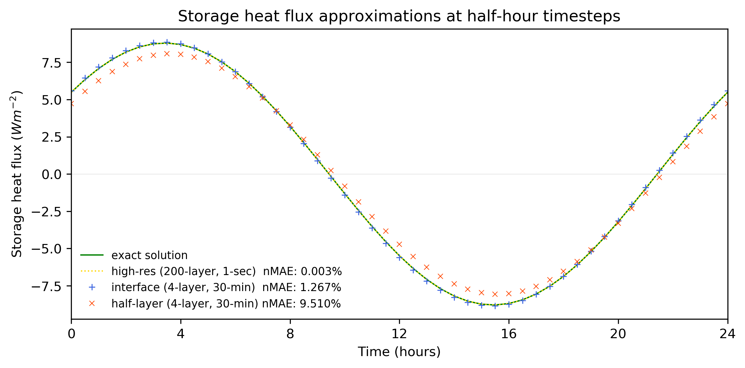
I have written Fortran code which solves conduction using the three methods described in this post. The program includes a check that energy is conserved. For further information on conduction schemes, refer to my post here, or journal paper here.

!!!!!!!!!!!!!!! conduction.f90 for Fortran 90 !!!!!!!!!!!!!!!!!!!!!!!!!!!!!!!!!!!!!!!!!!!!
! Purpose:      Three methods to simulate conduction through a multi-layered material
!               1. Half-layer scheme (standard method)
!               2. Modified half-layer scheme (standard method with additional surface node)
!               3. Interface scheme  method (proposed method)
!               4. Hgh resolution (Standard method witih 200 layers at 1 second timestep)
!               More information at https://www.theurbanist.com.au/2017/06/solving-the-heat-equation/
! Developer:    Mathew Lipson <m.lipson@unsw.edu.au>
! Revision:     27 Nov 2017
!!!!!!!!!!!!!!!!!!!!!!!!!!!!!!!!!!!!!!!!!!!!!!!!!!!!!!!!!!!!!!!!!!!!!!!!!!!!!!!!!!!!!!!!!!

program conduction
implicit none

integer, parameter :: dp = SELECTED_REAL_KIND(8)       ! double precision for energy closure check

type materialdata
  real(kind=dp), dimension(:,:), allocatable :: depth, volcp, lambda, nodetemp, nodetemp_prev
end type materialdata

real(kind=dp), dimension(:), allocatable :: temp_ext    ! external sol-air temperature (varying) [K]
real(kind=dp), dimension(:), allocatable :: temp_int    ! internal sol-air temperature (fixed )  [K]
real(kind=dp), dimension(:), allocatable :: storageflux ! total storage flux between timesteps   

real(kind=dp), parameter :: pi = 4 * atan (1.0_8) ! pi
real(kind=dp), parameter :: spinup = 10.          ! number of periods spin up to be discarded
integer, parameter :: ufull = 1                   ! number of tiles (for vectorisation)

real(kind=dp) :: ddt=1800.                        ! timestep length                         [s]
real(kind=dp) :: period=86400.                    ! sinusoidal period                       [s]
real(kind=dp) :: res_ext=0.04                     ! external surface resistance             [K m^2/W]  
real(kind=dp) :: res_int=0.13                     ! internal surface resistance             [K m^2/W]
integer :: nl = 4                                 ! number of layers in material            [-]
integer :: timesteps                              ! total timesteps in simulation           [-]
integer :: t                                      ! time loop integer
character(len=15) :: filename

integer, save :: conductmeth                      ! conduction method (0=half-layer, 1=interface)
type(materialdata), save :: material

print *, "Select conduction method (0=standard half-layer, 1=modified half-layer, 2=interface, 3=high-res): "
read *,conductmeth
write(filename, '(a,I0,a)') "output_",conductmeth,'.txt'
print *, "Writing to ", filename
open(1,file=filename,action="write",status="replace")
write(1,*) "timestep   temp_ext    storageflux nodetemp(0) nodetemp(1)"

! high-res standard half-layer run (exact)
if (conductmeth==3) then
  conductmeth=0
  nl = 200
  ddt = 1.
end if

allocate(material%depth(ufull,nl),material%volcp(ufull,nl),material%lambda(ufull,nl))
allocate(material%nodetemp(ufull,0:nl),material%nodetemp_prev(ufull,0:nl))
allocate(temp_ext(ufull),temp_int(ufull),storageflux(ufull))

! initialisation
timesteps = (int(spinup)+1)*(24*3600)/int(ddt)
material%nodetemp=290.                                            ! [K]
temp_ext = 290.                                                   ! [K]
temp_int = 290.                                                   ! [K]
! 4 layered wall
material%depth(1,:) =(/ 0.01, 0.04, 0.10, 0.05 /)                 ! [m]
material%volcp(1,:) =(/ 1.55E6, 1.55E6, 1.55E6, 0.29E6 /)         ! [J/m^3/K]
material%lambda(1,:)=(/ 0.9338, 0.9338, 0.9338, 0.0500 /)         ! [W/m/K]
! 200 layered wall (for high-res)
if (nl==200) then
  do t = 1,10
      material%depth(:,t)  = 0.001
      material%volcp(:,t)  = 1.55E6
      material%lambda(:,t) = 0.9338
  end do
  do t = 11,50
      material%depth(:,t)  = 0.001
      material%volcp(:,t)  = 1.55E6
      material%lambda(:,t) = 0.9338
  end do
  do t = 51,150
      material%depth(:,t)  = 0.001
      material%volcp(:,t)  = 1.55E6
      material%lambda(:,t) = 0.9338
  end do
  do t = 151,200
      material%depth(:,t)  = 0.001
      material%volcp(:,t)  = 0.29E6
      material%lambda(:,t) = 0.050
  end do
end if

! main loop
do t = 1, timesteps
  temp_ext = 290. + sin(2*pi*t*ddt/period)                        ! external temperature variation
  material%nodetemp_prev = material%nodetemp                      ! previous node temperatures
  call solvetridiag(temp_ext,temp_int,res_ext,res_int,ddt,     &       
                    material%nodetemp,                         &  ! layer temeperature
                    material%depth*material%volcp,             &  ! layer capacitance (cap)
                    material%depth/material%lambda)               ! layer resistance  (res)
  call energycheck(temp_ext,temp_int,res_ext,res_int,ddt,      &
                    material%nodetemp, material%nodetemp_prev, &  ! layer temeperature
                    material%depth*material%volcp,             &  ! layer capacitance (cap)
                    material%depth/material%lambda,            &  ! layer resistance  (res)
                    storageflux) 
  if ((t>=spinup*period/ddt) .and. MOD(t,1800/int(ddt))==0) then 
    write(1,'(I8,F12.4,F12.6,5F12.4)') t, temp_ext,storageflux, material%nodetemp(:,0:1)
  end if
end do

close(1)
deallocate(material%depth,material%volcp,material%lambda,material%nodetemp)
deallocate(material%nodetemp_prev,temp_ext,temp_int,storageflux)

contains

!!!!!!!!!!!!!!!!!!!!!!!!!!!!!!!!!!!!!!!!!!!!!!!!!!!!!!!!!!!!!!!!!!!!!
! Tridiagonal matrix form:
!  [ ggB ggC         ] [ nodetemp ] = [ ggD ]
!  [ ggA ggB ggC     ] [ nodetemp ] = [ ggD ]
!  [     ggA ggB ggC ] [ nodetemp ] = [ ggD ]
!  [         ggA ggB ] [ nodetemp ] = [ ggD ]

!  ufull is number of systems to be calculated (for vectorisation)
!  nl is number of layers in system
!  conductmeth is conduction method (standard half-layer=0, modified half-layer=1, interface=2)

subroutine solvetridiag(temp_ext,temp_int,res_ext,res_int,ddt,nodetemp,cap,res)

implicit none

real(kind=dp), dimension(ufull),     intent(in)    :: temp_ext,temp_int  ! boundary temperatures
real(kind=dp), dimension(ufull,0:nl),intent(inout) :: nodetemp           ! temperature of each node
real(kind=dp), dimension(ufull,nl),  intent(in)    :: cap,res            ! layer capacitance & resistance
real(kind=dp), intent(in)                          :: ddt                ! timestep
real(kind=dp), intent(in)                          :: res_ext,res_int    ! aerodynamic surface resistance

! local variables
real(kind=dp), dimension(ufull,0:nl)               :: ggA,ggB,ggC,ggD    ! tridiagonal matrices
real(kind=dp), dimension(ufull)                    :: ggX                ! tridiagonal coefficient
integer sidx ! index start integer
integer k  ! loop integer

select case(conductmeth)
  case(0) !!!!!!!!! standard half-layer conduction !!!!!!!!!!!
    sidx = 1
    ggA(:,2:nl)   =-2./(res(:,1:nl-1) +res(:,2:nl))
    ggB(:,1)      = 2./(2.*res_ext+ res(:,1))  +2./(res(:,1)+res(:,2)) + cap(:,1)/ddt
    ggB(:,2:nl-1) = 2./(res(:,1:nl-2) +res(:,2:nl-1)) +2./(res(:,2:nl-1) +res(:,3:nl)) +cap(:,2:nl-1)/ddt
    ggB(:,nl)     = 2./(res(:,nl-1)+res(:,nl)) + 1./(0.5*res(:,nl)+res_int) + cap(:,nl)/ddt
    ggC(:,1:nl-1) =-2./(res(:,1:nl-1)+res(:,2:nl))
    ggD(:,1)      = temp_ext/(res_ext+0.5*res(:,1)) + nodetemp(:,1)*cap(:,1)/ddt
    ggD(:,2:nl-1) = nodetemp(:,2:nl-1)*cap(:,2:nl-1)/ddt
    ggD(:,nl)     = nodetemp(:,nl)*cap(:,nl)/ddt + temp_int/(0.5*res(:,nl) + res_int)
  case(1) !!!!!!!!! modified half-layer conduction !!!!!!!!!!!
    sidx = 0
    ggA(:,1)      =-2./res(:,1)
    ggA(:,2:nl)   =-2./(res(:,1:nl-1) +res(:,2:nl))
    ggB(:,0)      = 2./res(:,1) +1./res_ext
    ggB(:,1)      = 2./res(:,1) +2./(res(:,1)+res(:,2)) + cap(:,1)/ddt
    ggB(:,2:nl-1) = 2./(res(:,1:nl-2) +res(:,2:nl-1)) +2./(res(:,2:nl-1) +res(:,3:nl)) +cap(:,2:nl-1)/ddt
    ggB(:,nl)     = 2./(res(:,nl-1)+res(:,nl)) + 1./(0.5*res(:,nl)+res_int) + cap(:,nl)/ddt
    ggC(:,0)      =-2./res(:,1)
    ggC(:,1:nl-1) =-2./(res(:,1:nl-1)+res(:,2:nl))
    ggD(:,0)      = temp_ext/res_ext
    ggD(:,1:nl-1) = nodetemp(:,1:nl-1)*cap(:,1:nl-1)/ddt
    ggD(:,nl)     = nodetemp(:,nl)*cap(:,nl)/ddt + temp_int/(0.5*res(:,nl) + res_int)
  case(2) !!!!!!!!! interface conduction !!!!!!!!!!!
    sidx = 0
    ggA(:,1:nl)   = -1./res(:,1:nl)
    ggB(:,0)      =  1./res(:,1) +1./res_ext +0.5*cap(:,1)/ddt
    ggB(:,1:nl-1) =  1./res(:,1:nl-1) +1./res(:,2:nl) +0.5*(cap(:,1:nl-1) +cap(:,2:nl))/ddt
    ggB(:,nl)     =  1./res(:,nl) +1./res_int +0.5*cap(:,nl)/ddt
    ggC(:,0:nl-1) = -1./res(:,1:nl)
    ggD(:,0)      = nodetemp(:,0)*0.5*cap(:,1)/ddt +temp_ext/res_ext
    ggD(:,1:nl-1) = nodetemp(:,1:nl-1)*0.5*(cap(:,1:nl-1)+cap(:,2:nl))/ddt
    ggD(:,nl)     = nodetemp(:,nl)*0.5*cap(:,nl)/ddt +temp_int/res_int
  case DEFAULT
    write(6,*) "ERROR: Unknown conduction mode selected: ",conductmeth
    stop
end select
! tridiagonal solver (Thomas algorithm) for node temperatures
do k=sidx+1,nl
  ggX(:)   = ggA(:,k)/ggB(:,k-1)
  ggB(:,k) = ggB(:,k)-ggX(:)*ggC(:,k-1)
  ggD(:,k) = ggD(:,k)-ggX(:)*ggD(:,k-1)
end do
nodetemp(:,nl) = ggD(:,nl)/ggB(:,nl)
do k=nl-1,sidx,-1
  nodetemp(:,k) = (ggD(:,k) - ggC(:,k)*nodetemp(:,k+1))/ggB(:,k)
end do

end subroutine solvetridiag

!!!!!!!!!!!!!!!!!!!!!!!!!!!!!!!!!!!!!!!!!!!!!!!!!!!!!!!!!!!!!!!!!!!!!!!!!!!!!!!!!!!!!!!!!
! conservation of energy: check for flux across boundaries matches change in heat storage

subroutine energycheck(temp_ext,temp_int,res_ext,res_int,ddt,nodetemp,nodetemp_prev,cap,res,storageflux)

implicit none

real(kind=dp), intent(in)                          :: res_ext,res_int        ! convective heat transfer
real(kind=dp), intent(in)                          :: ddt                    ! timestep
real(kind=dp), dimension(ufull),     intent(in)    :: temp_ext,temp_int      ! boundary temperatures
real(kind=dp), dimension(ufull,nl),  intent(in)    :: cap,res                ! layer capacitance & resistance
real(kind=dp), dimension(ufull,0:nl),intent(in)    :: nodetemp,nodetemp_prev ! temperature of each node
real(kind=dp), dimension(ufull),     intent(out)   :: storageflux            ! layer capacitance & resistance

! local variables
real(kind=dp), dimension(ufull) :: ggext,ggint,error

select case(conductmeth)
  case(0) !!!!!!!!! standard half-layer conduction !!!!!!!!!!!
    storageflux = sum((nodetemp(:,1:nl)-nodetemp_prev(:,1:nl))*cap(:,:), dim=2)/ddt
    ggext = (temp_ext-nodetemp(:,1))/(res_ext+0.5*res(:,1))
    ggint = (nodetemp(:,nl)-temp_int)/(0.5*res(:,nl)+res_int)
  case(1) !!!!!!!!! modified half-layer conduction !!!!!!!!!!!
    storageflux = sum((nodetemp(:,1:nl)-nodetemp_prev(:,1:nl))*cap(:,:), dim=2)/ddt
    ggext = (temp_ext-nodetemp(:,0))/res_ext
    ggint = (nodetemp(:,nl)-temp_int)/(0.5*res(:,nl)+res_int)
  case(2) !!!!!!!!! interface conduction !!!!!!!!!!!
    storageflux = sum((nodetemp(:,0:nl-1)-nodetemp_prev(:,0:nl-1))*0.5*cap(:,:), dim=2)/ddt   &
                 +sum((nodetemp(:,1:nl)  -nodetemp_prev(:,1:nl))  *0.5*cap(:,:), dim=2)/ddt
    ggext = (temp_ext-nodetemp(:,0))/res_ext
    ggint = (nodetemp(:,nl)-temp_int)/res_int
end select

error = (storageflux - (ggext - ggint))
! write(6,*) "closure error: ",error
if (any(abs(error)>1.E-6)) write(6,*) "closure error: ",error

end subroutine energycheck

!!!!!!!!!!!!!!!!!!!!!!!!!!!!!!!!!!!!!!!!!!!!!!!!!!!!!!!!!!!!!!!!!!!!!!!!!!!!

end program conduction

References

1. Lipson et al., 2017, Efficiently modelling urban heat storage: an interface conduction scheme in an urban land surface model (aTEB v2.0).
2. Recktenwald, Gerald W., Finite-difference approximations to the heat equation.