In a new paper¹, we introduce a method to simulate how heat is conducted through roofs, walls and roads. We show it improves the simulation of heat storage and release, a very important process in urban climate.

Urban climate models can help investigate which urban plans are most effective at reducing temperatures during heatwaves, or which conditions lead to high levels of air pollution, or predict spikes in building energy use, among other things. But cities are complex, and models must be simple. The trick is to find efficient modelling methods that are accurate enough for the processes you’re interested in.

One of the most important processes for urban climate is how heat is conducted through urban materials. When the sun beats down on a city, much of the energy is absorbed by concrete, asphalt and brick. At night those materials radiate heat back into the streets. This process is a key reason why city temperatures can be up to 10 °C warmer than natural surrounds².

But as it turns out, a lot models underestimate the magnitude of the heat moving between the atmosphere and urban materials³. We wanted to try to improve that.

In a paper¹ recently published in Geoscientific Model Development, Melissa Hart, Marcus Thatcher and I introduced a new method to calculate conduction through multilayered walls and roofs. We showed that our ‘interface’ conduction scheme is more accurate at lower resolutions, and therefore more efficient, compared with the method most commonly used in urban models today.

How we did it

A computer model takes the continuous equations describing the flow of energy and splits them into lumps for processing. This is called discretisation, and how we choose to divide a continuous three-dimensional world impacts on the accuracy and speed of a simulation.

The standard method

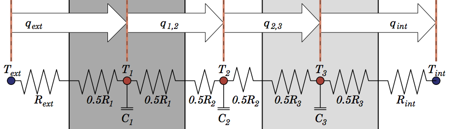
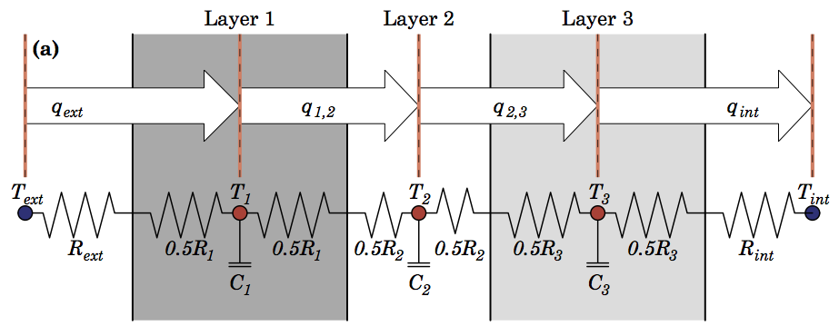
One method that is used in a lot of urban models to discretise walls and roofs is the half-layer scheme. It represents bulk capacitance at a node in the middle of a layer, thereby representing an average layer temperature. It’s most easily described graphically using the symbolism of an electrical circuit, where heat flow ($ q $) is regulated by a material’s heat resistance ($ R $), and capacitance ($ C $) regulates the energy required to increase a node’s temperature ($ T $):

The half-layer scheme is based on methods developed to simulate conduction through soil or snow, and it has been extensively evaluated in those instances. But I was interested in whether there was a better method for urban models, where walls and roofs are a combination of materials with sharply different thermal properties, as opposed to soil or snow properties which change gradually.

The interface scheme

As an alternative, we proposed a simple change to lump capacitance at the interface between layers:

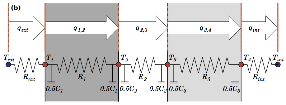
Having a capacitance/ temperature node at the surface of the system means external changes impact storage directly, rather than being mitigated through the resistance of the first half layer.

Both schemes can be described by different forms of the discretised one-dimensional heat diffusion equation (see Formulations below). Both introduce errors by chopping a continuous function into chunks of time and space. So to assess the schemes, we first compared errors with exact solutions in a highly controlled environment, and then put them in an urban climate model and compared output with observations in Melbourne.

Comparison with exact solutions

For a material with constant conductivity or heat capacity, the process of solving the heat equation analytically (i.e. exactly) are relatively straightforward. However calculating exact solutions for a material with step changes in thermal properties (a composite material) is less well known.

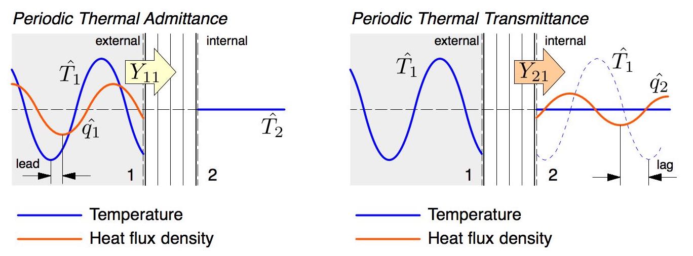
Here we used a technique called the admittance procedure, which calculates time-varying exact solutions to one-dimensional heat transfer for a system of materials exposed to a sinusoidal temperature variation on one side, fixed on the other. I like the method as it can quickly calculate a variety of important characteristics for composite materials that steady-state methods can not, like how much heat is absorbed at one surface and transmitted through the other over a day/night cycle. The mathematics are well laid out in an international standard ISO 13786:2007⁴.

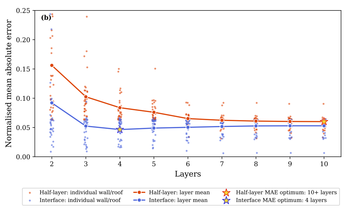
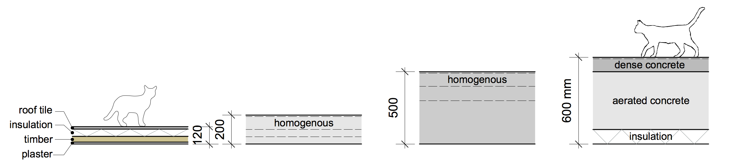
We used this to show that at resolutions typical of urban models, the interface scheme is better able to simulate the change in heat storage when tested against 32 common wall and roofs assemblies. The next step was to assess how this impacted an urban models ability to simulate climate by comparing with observations.

Comparison with observations

We compared model output with flux tower observations in Melbourne every 30 minutes for 16 months. We evaluated four different material set-ups and three different aerodynamic heat transfer formulations. The four materials set-ups were:

• SITE material properties based on surveys of the observation site
• WRF default material properties used in a popular urban model
• UZE properties which gave good results at a variety of sites worldwide
• aTEB properties which gave good results at a variety of sites in Australia

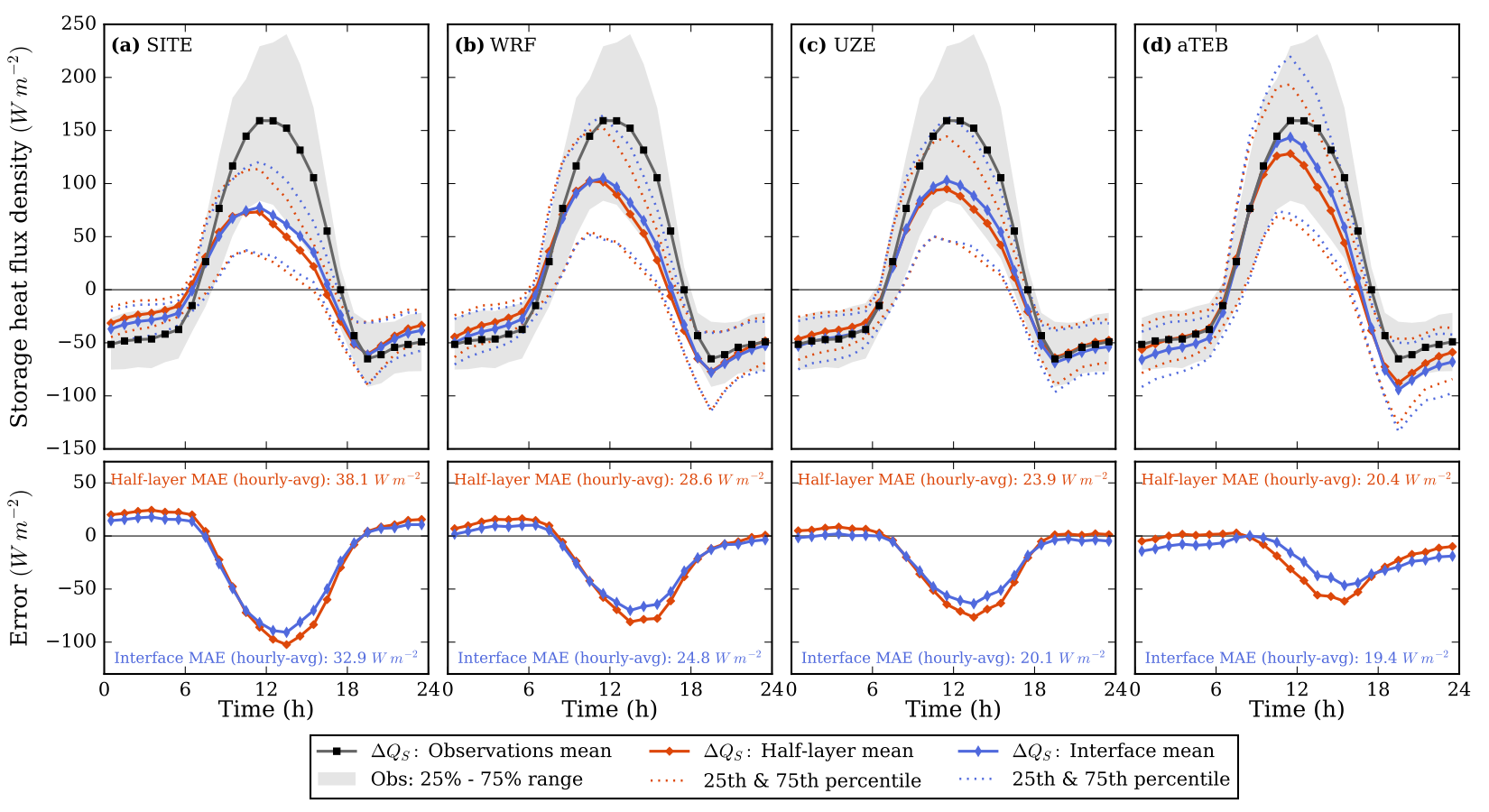
In each case the interface scheme reduced model errors for simulating heat storage, along with longwave and sensible heat fluxes. However, even in the best case errors were still quite large.

Frustratingly, the material set-up that performed the worst was the ‘realistic’ one, which most closely matched the site characteristics. This indicates that the simplifications used to make the model efficient has introduced biases that must be countered with unrealistic parameter choices.

This might be acceptable if we are studing processes in an existing city, where model parameters can be tuned so output matches observations. However for studies predicting processes in future cities, with different layouts, materials and climate regimes, then being able to use realistic material parameters becomes important.

So making a model that performs better with more realistic material choices is what I’m focussing on now. In the meantime, the interface scheme is an incremental improvement for our model, and might be beneficial to others too.

Formulations

The temperature evolution of node $k$ is described by a discretised one-dimensional heat equation:

$$ \tilde {C}_k \frac {T^{m+1}_k - T^m_k} {\Delta t} = \tilde {\kappa}_{k-1 \rightarrow } \left( T^{m+1}_{k-1} -T^{m+1}_k \right) - \tilde {\kappa}_{k \rightarrow} \left( T^{m+1}_k -T^{m+1}_{k+1} \right) $$

where $ \tilde {C} $ is effective heat capacitance of a node, $ T $ its temperature, $ m $ is timestep number, $ \Delta t $ timestep duration, and $ \tilde {\kappa}_{k \rightarrow} $ the effective conductance between nodes $k$ and $k+1$.

For the half-layer scheme, effective heat capacitance and conductance are:

$$ \begin{align} \tilde {C}_k &= c_i d_i \\
\tilde {\kappa}_{k \rightarrow} &= \left[ \frac{1}{2} \left( \frac{d_{i}}{ \lambda_{i}} + \frac{d_{i+1}}{ \lambda_{i+1}} \right) \right]^{-1} \end{align} $$

where $ d_i $ is the depth of the $i$th layer, $ c_i $ its volumetric heat capacity and $ \lambda_i $ its conductivity.

Then for the interface scheme:

$$ \begin{align} \tilde {C}_k &= \tfrac{1}{2} \left( c_{i-1} d_{i-1} + c_{i} d_{i} \right) \\
\tilde {\kappa}_{k \rightarrow} &= \frac {\lambda_i} {d_i} \end{align} $$

where $ c $ beyond boundaries of the system is zero (i.e. outer boundary nodes have only half the heat capacity of others).

These forms are fully implicit, meaning the updated temperature of a node is calculated simulataneously with other nodes in a matrix framework. This method is unconditionally stable, so we can use large timesteps without the program crashing (we use 30 minutes by default).

Code

Fortran code is available here which solves the above equations by decomposition and back-substitution in a tridiagonal matrix.

For an in depth explanation of the method, see here.

Key references

1. Lipson et al., 2017; Efficiently modelling urban heat storage: an interface conduction scheme in an urban land surface model (aTEB v2.0).
2. Santamouris, 2015; Analyzing the heat island magnitude and characteristics in one hundred Asian and Australian cities and regions.
3. Best and Grimmond, 2014; Key conclusions of the first international urban land surface model comparison project.
4. ISO 13786:2007; Thermal performance of building components – Dynamic thermal characteristics – Calculation methods.