Using machine learning to find an optimal model set-up

2017-09-12 · 1529 words · 8 minutes

code · workflow

AMALGAM · machine learning

I’ve recently finished developing a computational model which predicts the heating and cooling energy demands of a neighbourhood based on building characteristics, meteorological conditions and the behaviour of people. However, I don’t have a perfect and complete set of observations to describe the system, and I am finding it difficult to find appropriate values for some parameters. So I’ve used machine learning to help.

When testing how a model performs, we describe the thing we want to simulate with a series of model parameters which we believe match the real world, run the model, and then compare its predictions with observations. In describing the system, some model parameters are easy to measure, for example the height of a building or the material properties of asphalt. But others are more difficult. For my model, the average rate that air leaks from inside to outside the building was hard to quantify because of a lack of comprehensive observational data. This is obviously an important aspect for heating and cooling (anyone who’s lived in a leaky Australian house will agree!).

So what can do we do?

We first try to constrain parameters within a realistic range as best we can from site observations or other similar situations, and then undertake a series of simulations within that range and see how the model performs compared with observations we do have.

That’s fine when we have just a few parameters to test. However, when we have a larger number of parameters that are not tightly constrained, the number of simulations required to properly test the full ‘parameter space’ quickly increases to many thousands. Obviously analysing thousands of simulations is time consuming. On top of that, there are hundreds of different criteria we can use to assess the ‘best’ model set-up. So it can become very difficult to do in practical sense.

So what do we do next?

Machine learning?

We could try machine learning - computer algorithms which are programmed to recognise patterns and make decisions which lead to desired outcomes without being supervised. One such computer algorithm is AMALGAM, developed by Jasper Vrugt and Bruce Robinson. The code in MATLAB is available here.

AMALGAM is described as a set of evolutionary, multi-objective optimisation algorithms. Let’s try to break that down…

Evolutionary algorithms

A genetically adaptive or evolutionary algorithm uses biological natural selection as inspiration to find optimal solutions to a problem. The process is as follows:

An algorithm takes an initial set of, say, 100 individual model set-ups – together called a population. Each individual is described by a unique set of initially random parameter values within a set range (its genes).
The model is run, and each individual is assessed against set objectives and given a rank within that population across multiple criteria (its fitness).
A new generation of individuals (children) are created by mixing parameter values of similarly ranked parents, as well as randomly changing some or all of the parameter values (mutation).
Children are assessed for their fitness and compared with their parents. If the children are deemed ‘fitter’ they replace their parent, otherwise the parent’s genes are retained to contribute to the genes of the next generation.
The process is repeated for say, 100 generations, with the final generation taken as the fittest set of individuals.

Multi-objective optimisation – finding the Pareto front

Multi-objective optimisation is the process of finding a set of parameters that simultaneously minimise the error in multiple criteria. For example – two criteria could be the root mean square error of sensible heat flux and total electricity use. However, in complex problems, there is no single solution that simultaneously optimises all objectives. In other words, a subjective trade-off of performance is required.

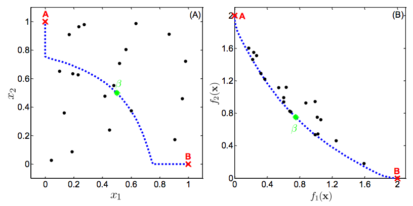
The set of solutions in which a single objective can not be further improved without degrading another is called the Pareto-optimal solution set, or the Pareto front. Without additional subjective preferences, all Pareto-optimal solutions are considered “equally good”. The point is illustrated in Figure 1.

$Figure 1 (by Jasper Vrugt): The left panel (a) shows a two-dimensional parameter space across $x_1$ and $x_2$, each with values between 0 and 1. Each dots represents an individual model set-up. The right panel (b) shows the results of each set up plotted against two objective criteria, $f_1$ and $f_2$. Point A is a model set up which minimises the $f_1$ objective, and point B is a set-up which minimises the $f_2$ objective. The blue dotted line is the Pareto-optimal set of solutions, with $\beta$ a member of the set and points lying off the line not optimal (for this set of objective criteria).$

AMALGAM – a ‘set’ of evolutionary, multi-objective algorithms

There are many algorithms that are both evolutionary and multi-objective. However, reliance on a single method of natural selection and adaptation can be problematic, as each method converges on the Pareto-optimal solution at different rates depending on the problem at hand.

AMALGAM combines multiple adaptation and selection methods with the intention of speeding up the process of convergence on the set of Pareto-optimal solutions. That is:

In each generation, the parent generation provide genes to children using different combination algorithms.
A new generation is selected based on fitness and by discarding individuals that are too similar to maintain a spread across the Pareto-front.
The the success of various combination methods is assessed, and those methods with higher reproductive success preferentially weighted in future generations.

Using this novel method of simultaneous genetic adaptive methods, AMALGAM claims to be a factor of 10 faster than other single-method optimisation algorithms.

How to use AMALGAM

AMALGAM is written in MATLAB and freely available from Jasper Vrugt’s website. I was able to get AMALGAM working in combination with my Fortran urban model within a few days thanks to good documentation and a helpful series of case-studies. I took one of the case-studies and adapted it for my needs.

I used a population of 50 individuals, over 100 generations, for a total of 5000 simulations. My urban model takes about 1 second to run for a 12-month simulation, so the total process takes about two hours (AMALGAM can be run in parallel over multiple processes, but I didn’t get this working).

I needed two MATLAB scripts.

The first script sets up the basic parameters of AMALGAM including the population and generation size, the number of parameters and their ranges, and various other options like how to save output. I simply adapted example_6.m from case study 6. I’ve included an example below of my first script.

%# Define fields of AMALGAMPar
AMALGAMPar.N = 50;                              %# Define population size
AMALGAMPar.T = 100;                             %# How many generations?
AMALGAMPar.d = 7;                               %# How many parameters?
AMALGAMPar.m = 3;                               %# How many objective functions?

%# Define fields of Par_info
Par_info.initial = 'latin';                     %# Latin hypercube sampling
Par_info.boundhandling = 'reflect';             %# Explicit boundary handling
Par_info.min = [1.00 1.0 0.5 283.0 288.0];      %# If 'latin', min values
Par_info.max = [20.0 5.0 4.0 293.0 298.0];      %# If 'latin', max values

%# Define name of function
Func_name = 'AMALGAM_ateb';

%# Define structure options
options.ranking = 'matlab';                     %# Example: Use Pareto ranking in matlab
options.print = 'yes'
options.save = 'yes'
options.restart = 'no'

%# Run the AMALGAM code and obtain non-dominated solution set
[X,F,output,Z] = AMALGAM(AMALGAMPar,Func_name,Par_info,options);

out=[X,F]
dlmwrite('M02_bm1_finalpop.csv',out)

The second script includes the call to a model, and the objective functions used to assess output. In my case I had to write out parameters to an external namelist file, then call my Fortran model, read back in the output and calculate the objective functions. This all seemed to work in a straightforward and efficient manner.

function [ F ] = AMALGAM_ateb ( x )

%# write parameters to namelist
%# filepath = '~/ownCloud/phd/03-Code/atebwrap';
filepath = '.';
Arun = 'M02';
%# namelist file
nmlfile = fopen('ateb.nml','wt');
fprintf(nmlfile, [...
	'&atebnml \n',...
	'/ \n',...
	'&atebsnow \n',...
	'/ \n',...
	'&atebgen \n',...
	'/ \n',...
	'&atebtile \n',...
	'/ \n',...
	'&atebtile \n',...
	'cinfilach  = %s,  2.0,  2.0,  2.0,  2.0,  2.0,  2.0,  2.0 \n',...
	'cventilach = %s,  4.0,  4.0,  4.0,  4.0,  0.5,  0.5,  0.5 \n',...
	'cintgains  = %s,  5.0,  5.0,  5.0,  5.0,  5.0,  5.0,  5.0 \n',...
	'ctempheat  = %s,  288.,  288.,  288.,  288.,  000.,  000.,  000. \n',...
	'ctempcool  = %s,  288.,  288.,  288.,  288.,  000.,  000.,  000. \n',...
	'/ \n'],x(1),x(2),x(3),x(4),x(5));
fclose(nmlfile);

EXP = sprintf('%s_bm1_acf%s_acc%s_inf%s_ven%s_ig_%s_ch%s_cc%s',Arun,x(1),x(2),x(3),x(4),x(5));

%# Run fortran code
fprintf('Running ateb experiment: %s',EXP)
system(sprintf('%s/atebwrap >variables.out',filepath));
system(sprintf('cp %s/energyout.dat %s/dummy.dat',filepath,filepath));

%# load simulation and observation starting after row[spinup], column[col], then
data = dlmread(sprintf('%s/energyout.dat',filepath),'',5205,8);
obs  = dlmread('obsQF.txt',',',[5205 6 22772 6]);

%# combine QF heating,cooling,base,traffic
datasum = data(:,1)+data(:,2)+data(:,3)+data(:,4);

%# Calculate objective functions
%# QF normalised standard deviation
F(1) = abs(1.0-std(datasum,'omitnan')/std(obs,'omitnan'));
%# QF correlation coefficient
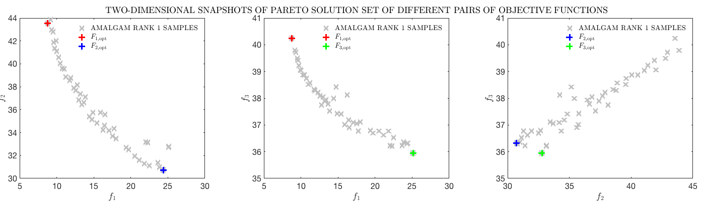
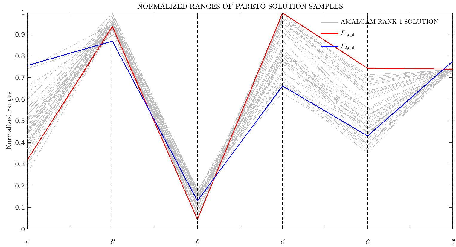
F(2) = 1.0-corr2(datasum,obs);

When finished, AMALGAM gives you a very fit population of individual model set-ups. It also plots a series of graphs showing you the shape of the Pareto front, how the fit population sits within the parameter space, how parameters are correlated.

Is this useful?

Overall, I think this is a really powerful tool for model development and exploration. I was able to reduce my RMSE in an important variable by about 20%. However, it would be a mistake to blindly trust the solutions that the method gives you. The solutions depend on the quality of the model, the quality of the observations we are comparing against, and the functions chosen to assess the model. In my case, my model is hardly a perfect representation of reality, and some of my observations are probably only accurate to about 20%.

What is useful is it can very efficiently scan the chosen parameter space to find the ranges of approprate parameter values, which can then feed into our understanding of which are the most important parameters to get right, and give a better idea of uncertainty in model predictions.

Example output

Figure 2: Example of Pareto-optimum solution in three objective functions

Figure 3: Example of optimum solution spread across paramater values